Deep Learning Hardware
CPU vs GPU
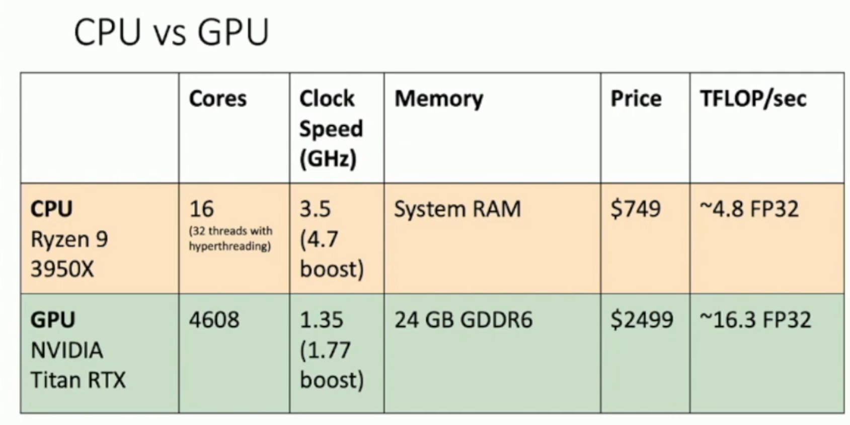
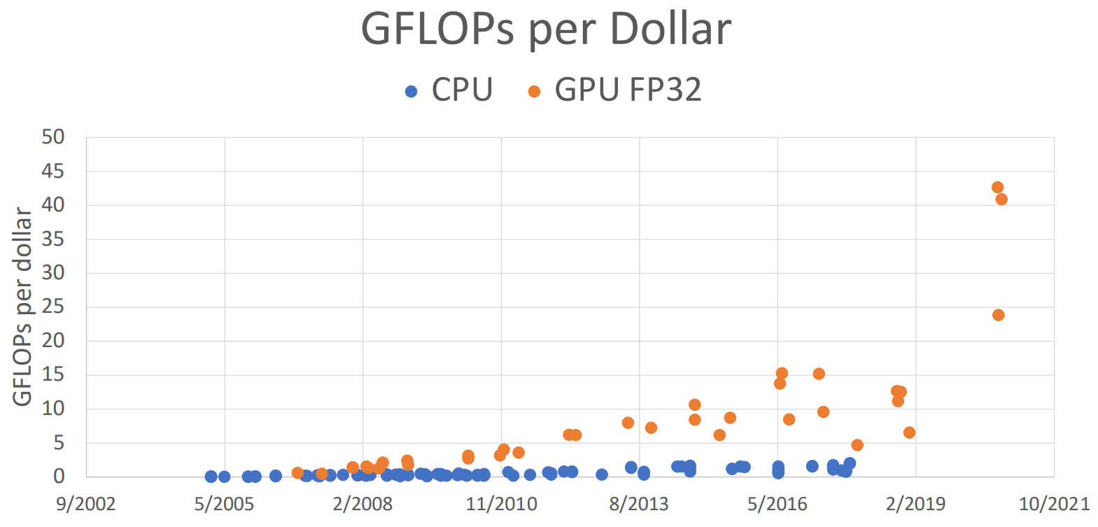
- The individual core of CPU is much faster, more powerful (i.e. better branch prediction, caching strategy) and more versatile than that of GPU (shown at the first graph)
- GPU have relatively "stupid" cores compared to CPUs, but it has a LOT of cores.
Inside a GPU: Titan
如上,
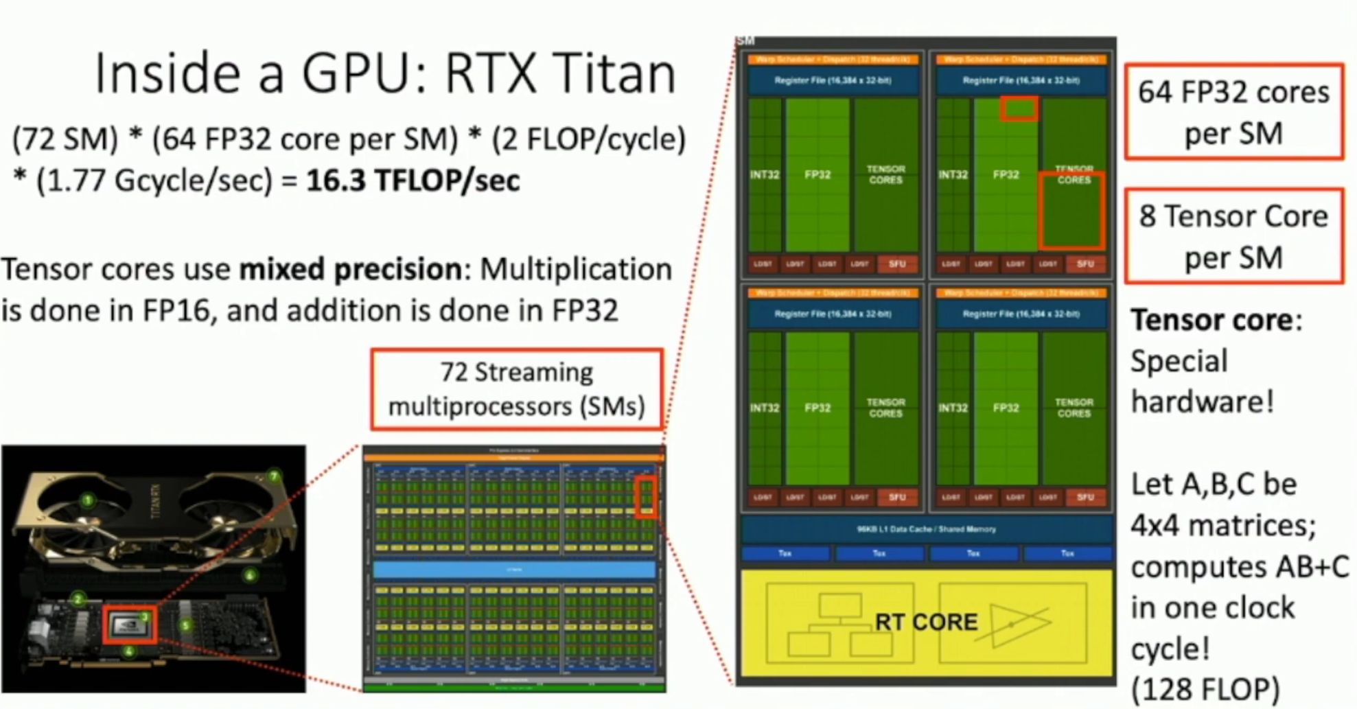
- 每一个 GPU 里,有 72 个 streaming multiprocessors (SMs)
- 每一个 SM 里,有 64 个 FP32 cores
- 每一个 FP32 Core,在一个 cycle 之内可以同时做乘法和加法,因此记作两次
- 同时,每一个 FP32 Core 的时钟频率为 1.77 Gcycle/sec
因此,虽然每一个 FP32 Core 很慢(性能只有 CPU 单核的百分之一不到),但是整体上是很快的。
Tensor core
另外,GPU 为了深度学习,还专门增添了 tensor core:在一个周期内,可以做到计算 \(AB+C\)。这需要
$$ FLOPS(A*B) + FLOPS(+C) = [(4 + 4 - 1) * 4 * 4] + [4 * 4] = 128 $$ 次浮点运算。
因此,如果考虑张量运算,就有:72 SM × 8 tensor cores per SM × 128 FLOPscycle × 1.77 Gcycle/sec ≈ 130.5 TFLOP
从而,GPU 的性能在矩阵乘法方面,比 CPU 强大得多。
Sidenote:
- 卷积操作可以转换成矩阵乘法,因此矩阵乘法对卷积操作非常 crucial
- 大矩阵可以视为小矩阵的分块乘法,因此可以用 4 × 4 矩阵乘法作为 subroutine
- 由于块与块之间是独立的,因此非常适合并行计算
- 如果大矩阵的边长不是 4 的倍数,那么可能就要 padding 等等,浪费性能,所以目前很多模型的矩阵大小都是 4 的倍数(实际上,都是 2 的次方数)
TPU
谷歌的 TPU 专门用于矩阵计算。在课程拍摄的时候(2019 年),PyTorch 还不支持 TPU,不过在 2024 年,早已经支持了(此处 TPU 被归为 XLA 设备)。
Deep Learning Software
Mainstream Learning Frameworks
Today, there are just two: PyTorch and Tensorflow.
Why do we need frameworks?
- Allow rapid prototyping of new ideas, i.e. it provides us with lots of common layers and utilities
- Auto-grad for us, i.e. it automatically use the computational graph to auto-grad, and we don't have to write our own code
- Run it efficiently on GPU/TPU/..., i.e. we don't have to deal with the very complicated interface of *PUs
PyTorch
PyTorch: Fundamental Concepts

Autograd
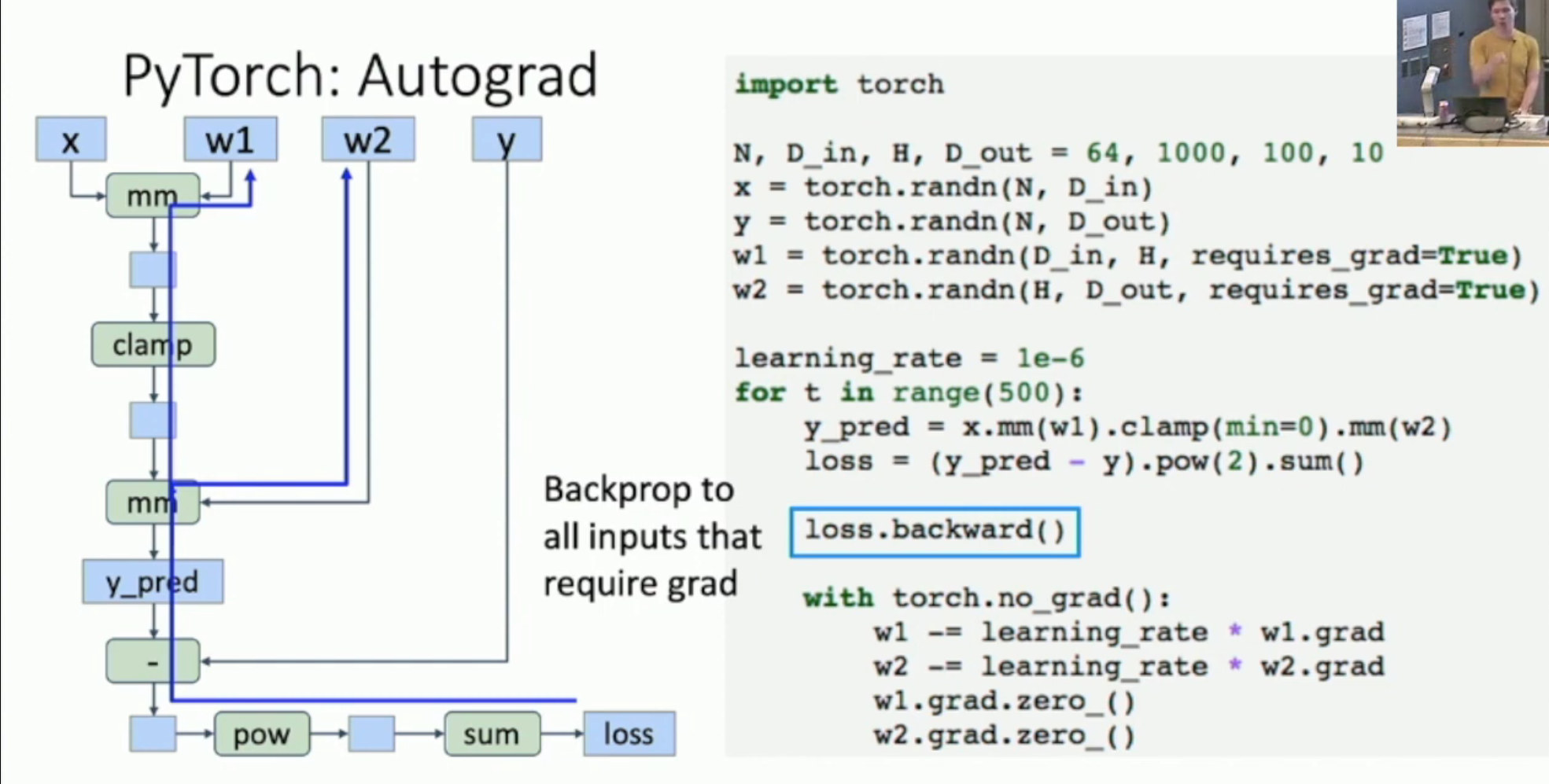
如图,PyTorch 的自动求导的方法如下:
- 你首先需要将希望求导的 tensor设置成
requires_grad=True - 然后,通过模块的叠加,算出最后的 loss。同时,PyTorch 隐式地自动构造出计算图(左图)
- 调用
loss.backward()- PyTorch 遍历所有设置了
requires_grad=True的模块 - 对于每一个这样的模块,PyTorch 找到通往这些模块的路径,然后进行自动求导
- 所有模块求导之后,PyTorch 会销毁计算图(同时释放计算图和反向传播占用的内存)
- 并且将计算结果存入各个
requires_grad=True的模块的grad
- PyTorch 遍历所有设置了
然后,我们需要在 torch.no_grad() 的环境下,
- 对 w1, w2 等进行更新
- 然后清空 w1, w2 的 grad:
w1.grad.zero_()- 否则,之后
loss.backward()存入 grad 的时候,就会加上之前遗留下来的 grad
- 否则,之后
New Functions
我们可以通过 python 的 function 构建新的函数,比如
但是,这样的构造方法,会使得 computation graph 如下图所示:
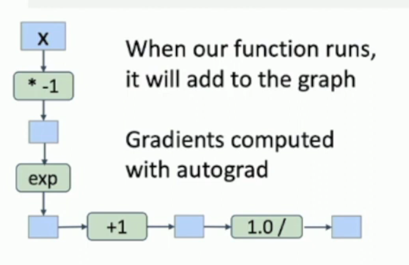
计算导数的时候,就是: $$ \newcommand{sgm}{\operatorname*{sigmoid}} \frac{\partial \sgm(x)}{\partial x} = \frac{\partial \sgm(x)}{\partial e^{-x}+1} \frac{\partial e^{-x}+1}{\partial e^{-x}} \frac{\partial e^{-x}}{\partial (-x)} \frac{\partial (-x)}{\partial x} = -\frac 1 { (e^{-x}+1)^2} * e^{-x} * -1 = \frac 1 {(e^{-x}+1)^2} * e^{-x} $$ 这样做就会导致计算量增加,且数值不稳定。
通常的做法是:\(\frac {\partial \sgm(x)} {\partial x} = \sgm(x) (1-\sgm(x))\)
而这样做,需要显式地告诉 PyTorch 导数是什么,因此,需要将 Sigmoid 通过一个派生类封装起来:
class Sigmoid(torch.autograd.Function):
    @staticmethod
    def forward(ctx, x):
        y = 1.0 / (1.0 + (-x).exp())
        ctx.save_for_backward(y)
        return y

    @staticmethod
    def backward(ctx, grad_y):
        y, = ctx.saved_tensors
        grad_x = grad_y * y * (1.0 - y)
        return grad_x

def sigmoid(x):
    return Sigmoid.apply(x)
- 当然,由于 \(\sgm\) 这种可以简便计算的函数并不多,因此我们通常还是使用 python 的函数。
- 只有求导可以用到 clever trick 的时候,再使用这种定义方式
Container
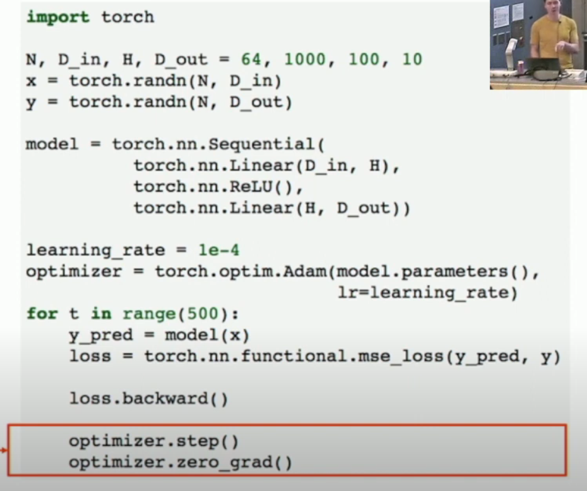
如图,我们将
- 各层封装成了一个 container (i.e.
torch.nn.Sequential)。这个 container 可以视作一个大型函数+一堆参数。 - 将梯度下降的工作交给了
optimizer去做- 可见在
torch.optim.Adam里,我们传入了model.parameter(),就是为了让 optimizer 自动帮我们进行梯度下降
- 可见在
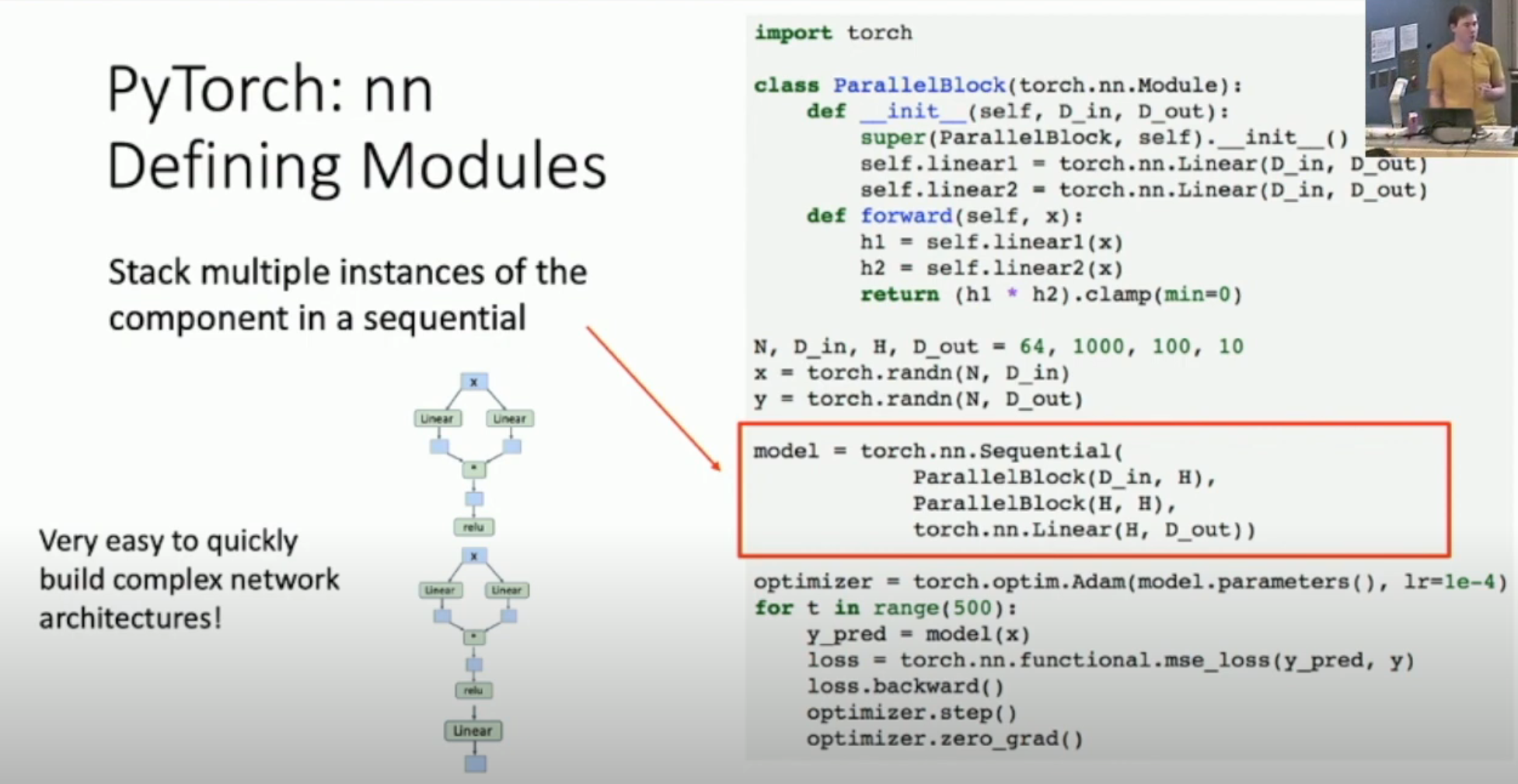
Module
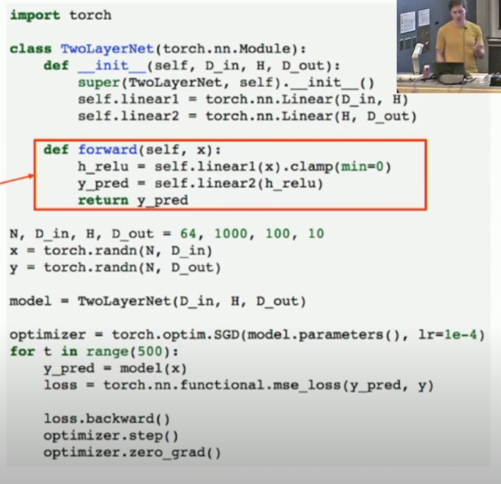
我们使用 module 来构建一个 network schema。然后还可以模块套模块,从而构建复杂的结构(如下图)。
Loader and Pre-trained Model
PyTorch 提供 loader,方便加载数据以及决定如何训练数据(比如 minibatch, shuffling, multithreading, etc);同时提供 pre-trained models,你可以直接调用,而 PyTorch 会从网络上下载。
PyTorch Advanced: Dynamic and Static Graph
Dynamic Graph
PyTorch 构建计算图的时候,默认采用 dynamic graph(如上文的代码),也就是——每次反向传播完毕之后,就销毁计算图,然后下一次迭代的时候重新构建。
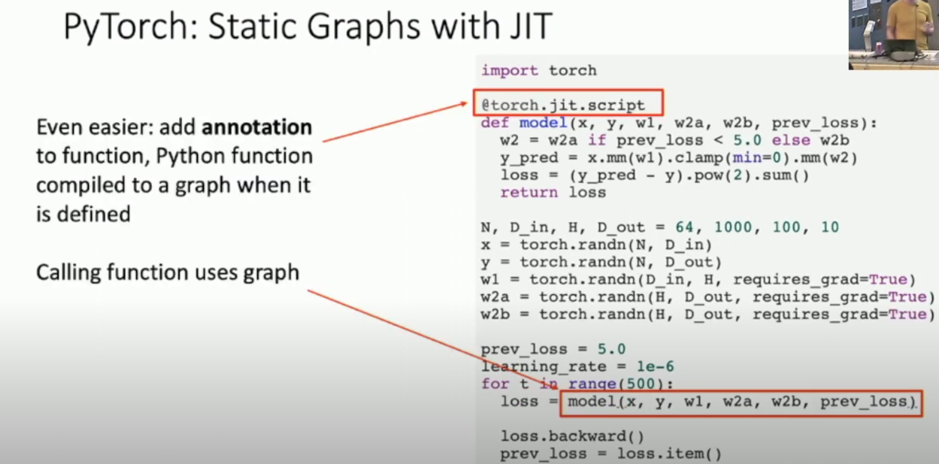
Static Graph
当然,这样的坏处就是:每一次你迭代的时候,都会有一个 overhead。为了避免这个 overhead,最新的 PyTorch 引入和 JIT 技术(如下图中的 @torch.jit.script 修饰符,或者用 graph = torch.jit.script(model)),可以即时编译出计算图。然后,你只需要每次迭代的时候,直接使用这个计算图即可,从而避免重复计算。
Pros and Cons
使用静态图的好处是:
- Reduce the overhead (of constructing naive graph, which we have mentioned)
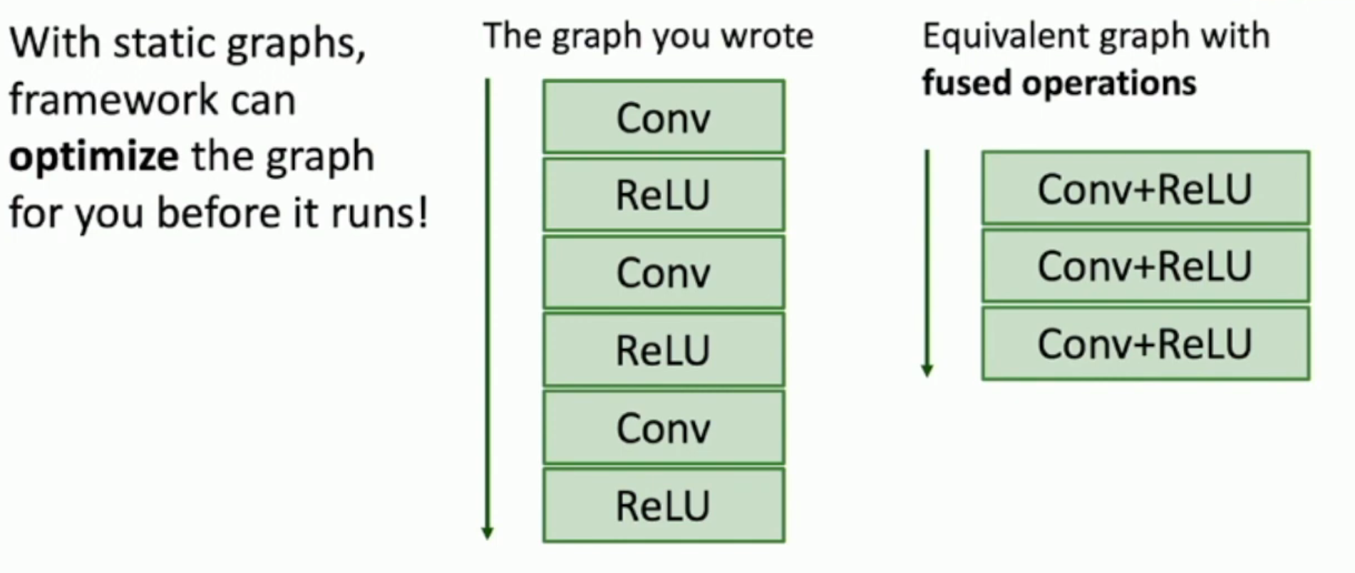
- Compile-time optimization (meaning the optimization overhead is also reduced)
- Once graph is built, can serialize it and run it without the code that built the graph! e.g. train model in Python,deploy in C++
使用静态图的坏处是:
- Lots of indirection between the code you write and the code that runs - can be hard to debug, benchmark, etc
使用动态图的好处是:
- 每一次迭代,也许你希望根据当前状态改变算式等等,从而动态图允许你动态改变算式
- The code you write is the code that runs! Easy to reason about, debug, profile, etc
使用动态图的坏处是:
- Graph building and executing is somewhat intertwined, so you always need to keep code around (i.e. train with Python interpreter, predict with it as well)
- This means, since they are intertwined, you can't extract the schema (i.e. the graph) from the code.
TensorFlow
TensorFlow 1.0 默认是 static graph。TensorFlow 2.0 默认是 dynamic graph。1.0 的 API 很乱,2.0 有很大改进。
另外,TensorBoard 作为可视化工具,非常美观且好用。PyTorch 也有一个接口:torch.utils.tensorboard。